Image Processing and Spatial linear transformations

We can think of an image as a function, f, from $\pmb R^2 \rightarrow R$ (or a 2D signal):

• f (x,y) gives the intensity at position (x,y)

Realistically, we expect the image only to be defined over a rectangle, with a finite range:
f: [a,b]x[c,d] -> [0,1]

A color image is just three functions pasted together. We can write this as a “vector-valued” function:

• Computing Transformations

If you have a transformation matrix you can evaluate the transformation that would be performed by multiplying the transformation matrix by the original array of points.

Examples of Transformations in 2D Graphics

In 2D graphics Linear transformations can be represented by 2x2 matrices. Most common transformations such as rotation, scaling, shearing, and reflection are linear transformations and can be represented in the 2x2 matrix. Other affine transformations can be represented in a 3x3 matrix.

Rotation

For rotation by an angle θ clockwise about the origin, the functional form is \( x’ = xcosθ + ysinθ \)
and \( y’ = − xsinθ + ycosθ \). Written in matrix form, this becomes:
$\begin{bmatrix} x' \cr \ y' \end{bmatrix} = \begin{bmatrix} \cos \theta & \sin\theta \cr \ -\sin \theta & \cos \theta \end{bmatrix} \begin{bmatrix} x \cr \ y \end{bmatrix}$

Scaling

For scaling we have \( x’; = s_x \cdot x \) and \( y’; = s_y \cdot y \). The matrix form is:
$\begin{bmatrix} x' \cr \ y' \end{bmatrix} = \begin{bmatrix} s_x & 0 \cr \ 0 & s_y \end{bmatrix} \begin{bmatrix} x \cr \ y \end{bmatrix}$

Shearing

For shear mapping (visually similar to slanting), there are two possibilities.
For a shear parallel to the x axis has \( x’; = x + ky \) and \( y’; = y \) ; the shear matrix, applied to column vectors, is:
$\begin{bmatrix} x' \cr \ y' \end{bmatrix} = \begin{bmatrix} 1 & k \cr \ 0 & 1 \end{bmatrix} \begin{bmatrix} x \cr \ y \end{bmatrix}$

A shear parallel to the y axis has \( x’; = x \) and \( y’; = y + kx \) , which has matrix form:
$\begin{bmatrix} x' \cr \ y' \end{bmatrix} = \begin{bmatrix} 1 & 0 \cr \ k & 1 \end{bmatrix} \begin{bmatrix} x \cr \ y \end{bmatrix}$

Image Processing

The package EBImage is an R package which provides general purpose functionality for the reading, writing, processing and analysis of images.

# source("http://bioconductor.org/biocLite.R")
# biocLite()
# biocLite("EBImage")
library(EBImage)

# Reading Image
img <- readImage("images/lena_std.tif")

#str(img1)
dim(img)

## [1] 512 512   3

display(img, method = "raster")

Image Properties

Images are stored as multi-dimensional arrays containing the pixel intensities. All EBImage functions are also able to work with matrices and arrays.

print(img)

## Image 
##   colorMode    : Color 
##   storage.mode : double 
##   dim          : 512 512 3 
##   frames.total : 3 
##   frames.render: 1 
## 
## imageData(object)[1:5,1:6,1]
##           [,1]      [,2]      [,3]      [,4]      [,5]      [,6]
## [1,] 0.8862745 0.8862745 0.8862745 0.8862745 0.8862745 0.8901961
## [2,] 0.8862745 0.8862745 0.8862745 0.8862745 0.8862745 0.8901961
## [3,] 0.8745098 0.8745098 0.8745098 0.8745098 0.8745098 0.8901961
## [4,] 0.8745098 0.8745098 0.8745098 0.8745098 0.8745098 0.8705882
## [5,] 0.8862745 0.8862745 0.8862745 0.8862745 0.8862745 0.8862745

• Adjusting Brightness

img1 <- img + 0.2
img2 <- img - 0.3
display(img1, method = "raster")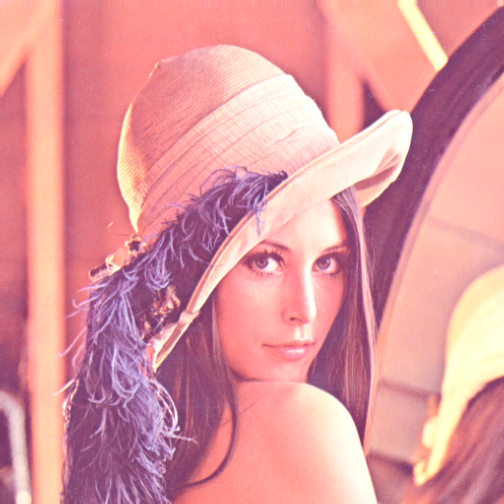

display(img2, method = "raster")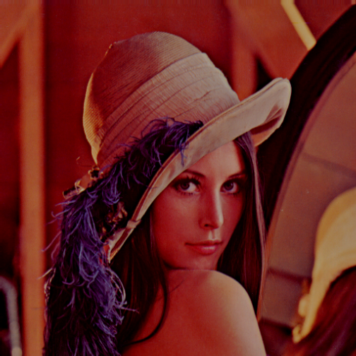

• Adjusting Contrast

img1 <- img * 0.5
img2 <- img * 2
display(img1, method = "raster")

display(img2, method = "raster")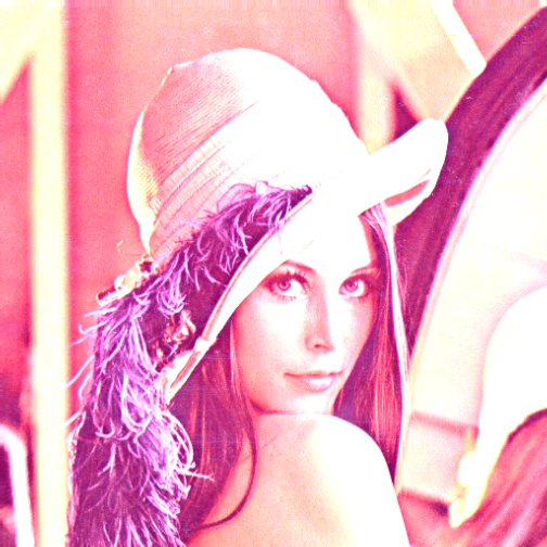

• Gamma Correction

img1 <- img ^ 4
img2 <- img ^ 0.9
img3 <- (img + 0.2) ^3
display(img1, method = "raster")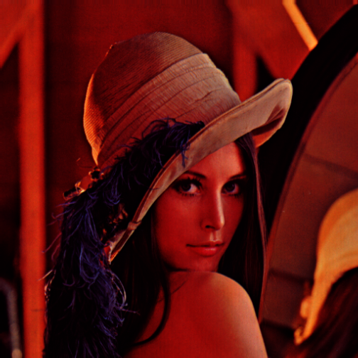

display(img2, method = "raster")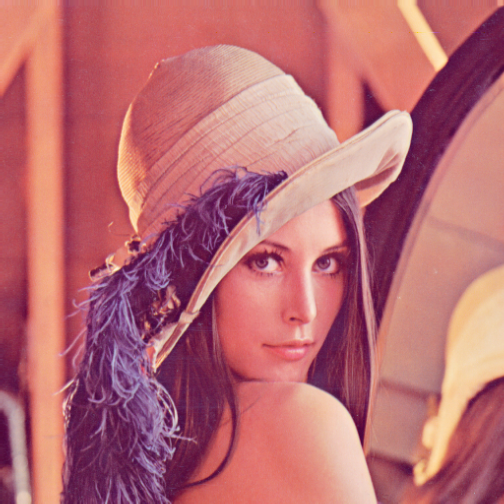

display(img3, method = "raster")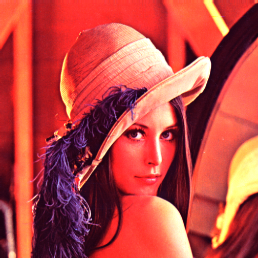

• Cropping Image

img1 <-img[(1:400)+100, 1:400,]
display(img1, method = "raster")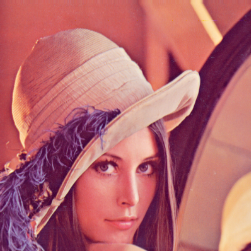

Spatial Transformation

Spatial image transformations are done with the functions resize, rotate, translate and the functions flip and flop to reflect images.

Next we show the functions flip, flop, rotate and translate:

y <- flip(img)
display(y, title='flip(img)', method = "raster")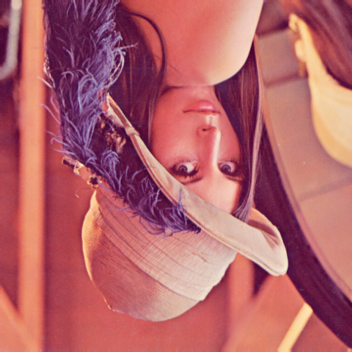

y = flop(img) 
display(y, title='flop(img)', method = "raster")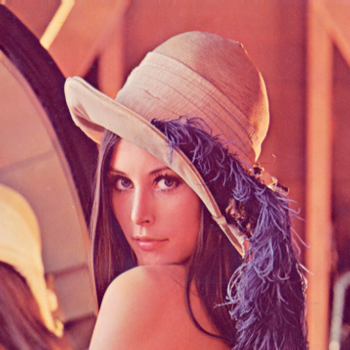

y <- rotate(img, 30) 
display(y, title='rotate(img, 30)', method = "raster")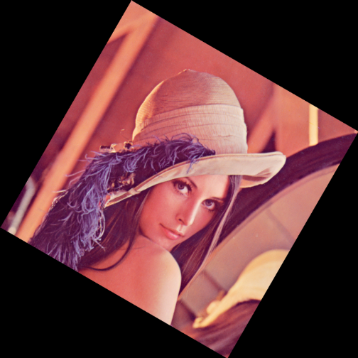

y <- translate(img, c(120, -20)) 
display(y, title='translate(img, c(120, -20))', method = "raster")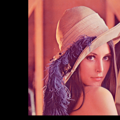

All spatial transforms except flip and flop are based on the general affine transformation.

Linear transformations using the function affine:

• Horizontal flip

m <- matrix(c(-1, 0, 0, 1, 512, 0), nrow=3,  ncol=2, byrow = TRUE)
m  # Horizontal flip

##      [,1] [,2]
## [1,]   -1    0
## [2,]    0    1
## [3,]  512    0

display(affine(img, m),  method = "raster")

• Horizontal shear ${m} = \left[ \begin{array}{cc} 1, 1/2 \cr \\ 0, 1 \end{array} \right]$

m <- matrix(c(1, 1/2, 0, 1, 0, -100), nrow=3,  ncol=2, byrow = TRUE)
m  # horizontal shear  r = 1/2 

##      [,1]   [,2]
## [1,]    1    0.5
## [2,]    0    1.0
## [3,]    0 -100.0

display(affine(img, m),  method = "raster")

• Rotation by π/6 ${m} = \left[ \begin{array}{cc} cos(pi/6), -sin(pi/6) \cr \\ sin(pi/6), cos(pi/6) \end{array} \right]$

m <- matrix(c(cos(pi/6), -sin(pi/6), sin(pi/6) , cos(pi/6), -100, 100), nrow=3,  ncol=2, byrow = TRUE)
m  # Rotation by π/6

##              [,1]        [,2]
## [1,]    0.8660254  -0.5000000
## [2,]    0.5000000   0.8660254
## [3,] -100.0000000 100.0000000

display(affine(img, m),  method = "raster")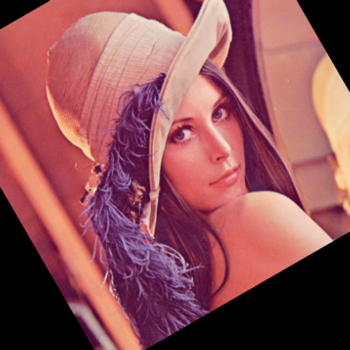

• Squeeze mapping with r=3/2 ${m} = \left[ \begin{array}{cc} 3/2, 0 \cr \\ 0, 2/3 \end{array} \right]$

m <- matrix(c(3/2, 0, 0, 2/3, 0, 100), nrow=3,  ncol=2, byrow = TRUE)
m  # Squeeze mapping with r=3/2

##      [,1]        [,2]
## [1,]  1.5   0.0000000
## [2,]  0.0   0.6666667
## [3,]  0.0 100.0000000

display(affine(img, m),  method = "raster")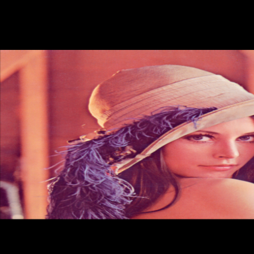

• Scaling by a factor of 3/2 ${m} = \left[ \begin{array}{cc} 3/2, 0 \cr \\ 0, 3/2 \end{array} \right]$

m <- matrix(c(3/2, 0, 0, 3/2, -100, -100), nrow=3,  ncol=2, byrow = TRUE)
m  # Scaling by a factor of 3/2

##        [,1]   [,2]
## [1,]    1.5    0.0
## [2,]    0.0    1.5
## [3,] -100.0 -100.0

display(affine(img, m),  method = "raster")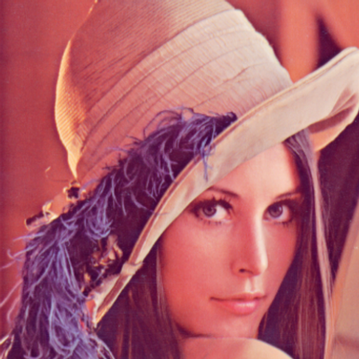

• Scaling horizontally by a factor of 1/2 ${m} = \left[ \begin{array}{cc} 1/2, 0 \cr \\ 0, 1 \end{array} \right]$

m <- matrix(c(1/2, 0, 0, 1, 0, 0), nrow=3,  ncol=2, byrow = TRUE)
m  # scale a figure horizontally  r = 1/2 

##      [,1] [,2]
## [1,]  0.5    0
## [2,]  0.0    1
## [3,]  0.0    0

display(affine(img, m),  method = "raster")

References

• http://www.iitg.ernet.in/scifac/qip/public_html/cd_cell/chapters/dig_image_processin.pdf
• http://www.math.ksu.edu/research/i-center/UndergradScholars/manuscripts/FernandoRoman.pdf
• http://www.statpower.net/Content/310/R%20Stuff/SampleMarkdown.html
• http://linear.ups.edu/html/section-LT.html
• http://www.r-bloggers.com/r-image-analysis-using-ebimage/
• http://www.maa.org/external_archive/joma/Volume8/Kalman/Linear3.html
• https://en.wikipedia.org/wiki/Linear_map
• https://en.wikipedia.org/wiki/Matrix_%28mathematics%29
• https://en.wikipedia.org/wiki/Affine_transformation
• http://mathforum.org/mathimages/index.php/Transformation_Matrix