MRI image segmentation

Magnetic Resonance Imaging (MRI) is a medical image technique used to sense the irregularities in human bodies. Segmentation technique for Magnetic Resonance Imaging (MRI) of the brain is one of the method used by radiographer to detect any abnormality happened specifically for brain.

In digital image processing, segmentation refers to the process of splitting observe image data to a serial of non-overlapping important homogeneous region. Clustering algorithm is one of the process in segmentation.
Clustering in pattern recognition is the process of partitioning a set of pattern vectors in to subsets called clusters.

There are various image segmentation techniques based on clustering. One example is the K-means clustering.

Image Segmentation

Let’s try the Hierarchial clustering with an MRI image of the brain.
The healthy data set consists of a matrix of intensity values.

healthy = read.csv("healthy.csv", header=FALSE)
healthyMatrix = as.matrix(healthy)
str(healthyMatrix)

##  num [1:566, 1:646] 0.00427 0.00855 0.01282 0.01282 0.01282 ...
##  - attr(*, "dimnames")=List of 2
##   ..$ : NULL
##   ..$ : chr [1:646] "V1" "V2" "V3" "V4" ...

# Plot image
image(healthyMatrix,axes=FALSE,col=grey(seq(0,1,length=256)))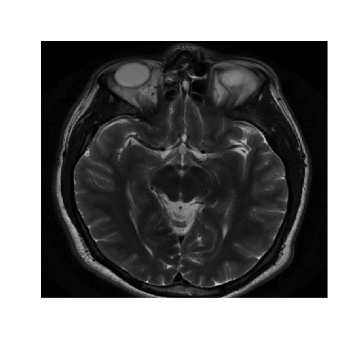

To use hierarchical clustering we first need to convert the healthy matrix to a vector. And then we need to compute the distance matrix.

# Hierarchial clustering
healthyVector = as.vector(healthyMatrix)
distance = dist(healthyVector, method = "euclidean")

## Error: cannot allocate vector of size 498.0 Gb

R gives us an error that seems to tell us that our vector is huge, and R cannot allocate enough memory.

Let’s see the structure of the healthy vector.

str(healthyVector)

##  num [1:365636] 0.00427 0.00855 0.01282 0.01282 0.01282 ...

n <- 365636

The healthy vector has 365636 elements. Let’s call this number n. For R to calculate the pairwise distances, it would need to calculate n*(n-1)/2 and store them in the distance matrix.
This number is 6.6844659 × 10¹⁰. So we cannot use hierarchical clustering.

Now let’s try use the k-means clustering algorithm, that aims at partitioning the data into k clusters, in a way that each data point belongs to the cluster whose mean is the nearest to it.

# Specify number of clusters.
# Our clusters would ideally assign each point in the image to a tissue class or a particular substance, for instance, grey matter or white matter, and so on. And these substances are known to the medical community. So setting the number of clusters depends on exactly what you're trying to extract from the image.
k = 5

# Run k-means
set.seed(1)
KMC = kmeans(healthyVector, centers = k, iter.max = 1000)
str(KMC)

## List of 9
##  $ cluster     : int [1:365636] 3 3 3 3 3 3 3 3 3 3 ...
##  $ centers     : num [1:5, 1] 0.4818 0.1062 0.0196 0.3094 0.1842
##   ..- attr(*, "dimnames")=List of 2
##   .. ..$ : chr [1:5] "1" "2" "3" "4" ...
##   .. ..$ : NULL
##  $ totss       : num 5775
##  $ withinss    : num [1:5] 96.6 47.2 39.2 57.5 62.3
##  $ tot.withinss: num 303
##  $ betweenss   : num 5472
##  $ size        : int [1:5] 20556 101085 133162 31555 79278
##  $ iter        : int 2
##  $ ifault      : int 0
##  - attr(*, "class")= chr "kmeans"

# Extract clusters
healthyClusters = KMC$cluster
KMC$centers[2]

## [1] 0.1061945

Analyze the clusters

To output the segmented image we first need to convert the vector healthy clusters to a matrix.
We will use the dimension function, that takes as an input the healthyClusters vector. We turn it into a matrix using the combine function, the number of rows, and the number of columns that we want.

# Plot the image with the clusters
dim(healthyClusters) = c(nrow(healthyMatrix), ncol(healthyMatrix))

image(healthyClusters, axes = FALSE, col=rainbow(k))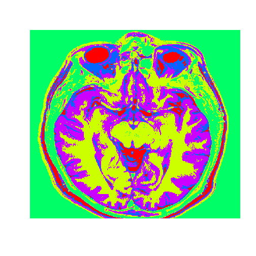

Now we will use the healthy brain vector to analyze a brain with a tumor

The tumor.csv file corresponds to an MRI brain image of a patient with oligodendroglioma, a tumor that commonly occurs in the front lobe of the brain. Since brain biopsy is the only definite diagnosis of this tumor, MRI guidance is key in determining its location and geometry.

Now, we will apply the k-means clustering results that we found using the healthy brain image on the tumor vector. To do this we use the flexclust package.
The flexclust package contains the object class KCCA, which stands for K-Centroids Cluster Analysis. We need to convert the information from the clustering algorithm to an object of the class KCCA.

# Apply to a test image
 
tumor = read.csv("tumor.csv", header=FALSE)
tumorMatrix = as.matrix(tumor)
tumorVector = as.vector(tumorMatrix)

# Apply clusters from before to new image, using the flexclust package
#install.packages("flexclust")
library(flexclust)

KMC.kcca = as.kcca(KMC, healthyVector)
tumorClusters = predict(KMC.kcca, newdata = tumorVector)

# Visualize the clusters
dim(tumorClusters) = c(nrow(tumorMatrix), ncol(tumorMatrix))

f <- function(m) t(m)[,nrow(m):1] # function to rotate our matrix 90 degrees clockwise
tumorClusters <- f(tumorClusters) # rotation achieved by our function


image((tumorClusters), axes = FALSE, col=rainbow(k), useRaster=TRUE)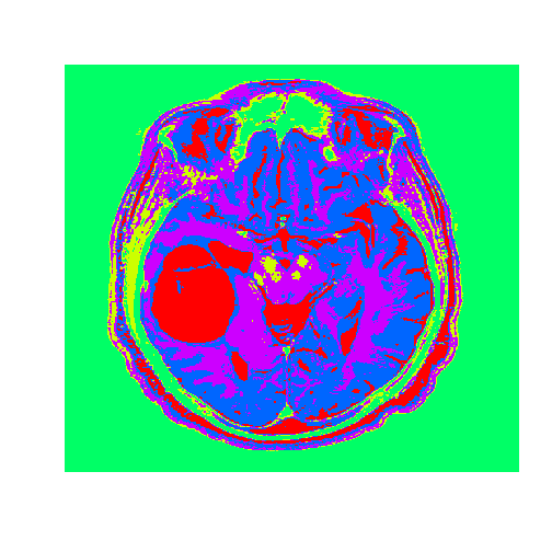

The tumor is the abnormal substance here that is highlighted in red that was not present in the healthy MRI image.

References

• https://www.edx.org/course/analytics-edge-mitx-15-071x-0
• https://courses.cs.washington.edu/courses/cse576/book/ch10.pdf
• http://blog.snap.uaf.edu/2012/06/08/matrix-rotation-for-image-and-contour-plots-in-r/
• http://www.cynthiaodonnell.com/2015/04/clustering/