Statistical Inference

Introduction

This is the project for the statistical inference class. In it, you will use simulation to explore inference and do some simple inferential data analysis. The project consists of two parts:

1. A simulation exercise.
2. Basic inferential data analysis.

Simulation exercises

The exponential distribution can be simulated in R with rexp(n, lambda) where lambda is the rate parameter. The mean of exponential distribution is 1/lambda and the standard deviation is also 1/lambda. Set lambda = 0.2 for all of the simulations. You will investigate the distribution of averages of 40 exponentials. Note that you will need to do a thousand simulations.

set.seed(33)
lambda <- 0.2
# We perform 1000 simulations with 40 samples 
sample_size <- 40
simulations <- 1000

# Lets do 1000 simulations
simulated_exponentials <- replicate(simulations, mean(rexp(sample_size,lambda)))
# 
simulated_means  <- mean(simulated_exponentials)
simulated_median <- median(simulated_exponentials)
simulated_sd     <- sd(simulated_exponentials)

Results

1. Show the sample mean and compare it to the theoretical mean of the distribution.

The theoretical mean and sample mean for the exponential distribution.

tm <- 1/lambda                     # calculate theoretical mean
sm <- mean(simulated_exponentials) # calculate avg sample mean

Theoretical mean: 5

Sampling mean: 4.9644306

The sample mean is very close to the theoretical mean at 5.

hist(simulated_exponentials,  freq=TRUE, breaks=50,
     main="Sample Means of Exponentials (lambda 0.2)",
     xlab="Sample Means from 1000 Simulations")
abline(v=5, col="blue", lwd=2)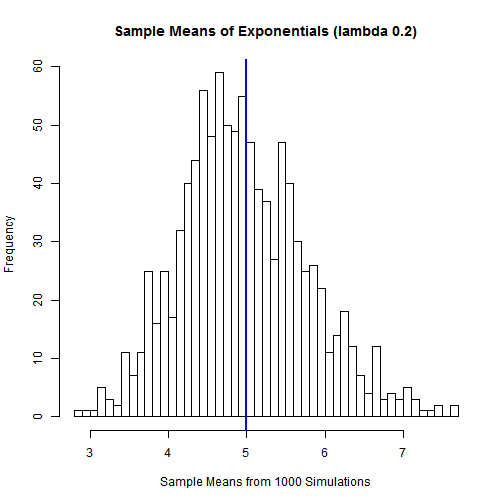

2. Show how variable the sample is (via variance) and compare it to the theoretical variance of the distribution.

# Calculation of the theoretical sd
theor_sd <- (1/lambda)/sqrt(40)
# Calculation of the theoretical variance for sampling data
theor_var <- theor_sd^2

simulated_var    <- var(simulated_exponentials)

The variance for the sample data is : 0.6456619 and the theoretical variance is : 0.625 Both these values are quite close to each other.

3. Show that the distribution is approximately normal.

qqnorm(simulated_exponentials, ylab = "Sample Means of Exponentials (lambda 0.2)")
qqline(simulated_exponentials, col = 2)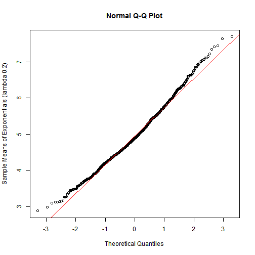

we see that the distribution is approximately normal as the straight line is closer to the points.