
MITx: 15.071x The Analytics Edge
31 May 2015Predicting loan repayment and Risk
In the lending industry, investors provide loans to borrowers in exchange for the promise of repayment with interest. If the borrower repays the loan, then the lender profits from the interest. However, if the borrower is unable to repay the loan, then the lender loses money. Therefore, lenders face the problem of predicting the risk of a borrower being unable to repay a loan.
1. Preparing the Dataset
Load the dataset loans.csv into a data frame called loans, and explore it using the str() and summary() functions. What proportion of the loans in the dataset were not paid in full? Please input a number between 0 and 1.
loans <- read.csv("data/loans.csv")
str(loans)
## 'data.frame': 9578 obs. of 14 variables:
## $ credit.policy : int 1 1 1 1 1 1 1 1 1 1 ...
## $ purpose : Factor w/ 7 levels "all_other","credit_card",..: 3 2 3 3 2 2 3 1 5 3 ...
## $ int.rate : num 0.119 0.107 0.136 0.101 0.143 ...
## $ installment : num 829 228 367 162 103 ...
## $ log.annual.inc : num 11.4 11.1 10.4 11.4 11.3 ...
## $ dti : num 19.5 14.3 11.6 8.1 15 ...
## $ fico : int 737 707 682 712 667 727 667 722 682 707 ...
## $ days.with.cr.line: num 5640 2760 4710 2700 4066 ...
## $ revol.bal : int 28854 33623 3511 33667 4740 50807 3839 24220 69909 5630 ...
## $ revol.util : num 52.1 76.7 25.6 73.2 39.5 51 76.8 68.6 51.1 23 ...
## $ inq.last.6mths : int 0 0 1 1 0 0 0 0 1 1 ...
## $ delinq.2yrs : int 0 0 0 0 1 0 0 0 0 0 ...
## $ pub.rec : int 0 0 0 0 0 0 1 0 0 0 ...
## $ not.fully.paid : int 0 0 0 0 0 0 1 1 0 0 ...table(loans$not.fully.paid)##
## 0 1
## 8045 1533tb <- table(loans$not.fully.paid)[2]/sum(table(loans$not.fully.paid))- ANS: 0.1600543
Explanation </br> From table(loans$not.fully.paid), we see that 1533 loans were not paid, and 8045 were fully paid. Therefore, the proportion of loans not paid is 1533/(1533+8045)=0.1601.
Using a revised version of the dataset that has the missing values filled in with multiple imputation.
#library(mice)
set.seed(144)
# vars.for.imputation = setdiff(names(loans), "not.fully.paid")
# imputed = complete(mice(loans[vars.for.imputation]))
# loans[vars.for.imputation] = imputed
# loans[vars.for.imputation]
loans <- read.csv("data/loans_imputed.csv")
2. Prediction Models
1. Now that we have prepared the dataset, we need to split it into a training and testing set. To ensure everybody obtains the same split, set the random seed to 144 (even though you already did so earlier in the problem) and use the sample.split function to select the 70% of observations for the training set (the dependent variable for sample.split is not.fully.paid). Name the data frames train and test. Now, use logistic regression trained on the training set to predict the dependent variable not.fully.paid using all the independent variables.
-
Which independent variables are significant in our model? (Significant variables have at least one star, or a Pr(> z ) value less than 0.05.) Select all that apply.
library(caTools)
set.seed(144)
split = sample.split(loans$not.fully.paid, SplitRatio = 0.70)
train = subset(loans, split== TRUE)
test = subset(loans, split== FALSE)

model0 <-glm(not.fully.paid ~. , data = train, family = "binomial")
# summary(model0)
Variables that are significant have at least one star in the coefficients table of the summary(model0) output. Note that some have a positive coefficient (meaning that higher values of the variable lead to an increased risk of defaulting) and some have a negative coefficient (meaning that higher values of the variable lead to a decreased risk of defaulting).
2. Consider two loan applications, which are identical other than the fact that the borrower in Application A has FICO credit score 700 while the borrower in Application B has FICO credit score 710. Let Logit(A) be the log odds of loan A not being paid back in full, according to our logistic regression model, and define Logit(B) similarly for loan B.
- Logit = belta’*x
- Logit(A) - Logit(B) = belta’*(x(A)-x(B))
logA=9.260+(-9.406e-03*700)
logB=9.260+(-9.406e-03*710)
ans1 <- logA - logB
ans1
## [1] 0.09406-
What is the value of Logit(A) - Logit(B)?
-
ANS: 0.09406
Now, let O(A) be the odds of loan A not being paid back in full, according to our logistic regression model, and define O(B) similarly for loan B. What is the value of O(A)/O(B)? (HINT: Use the mathematical rule that exp(A + B + C) = exp(A)exp(B)exp(C). Also, remember that exp() is the exponential function in R.) </br>
ans2 <- exp(logA)/exp(logB)
ans2
## [1] 1.098626-
What is the value of O(A)/O(B)?
-
ANS: 1.0986257
3. Prediction Models
1. Predict the probability of the test set loans not being paid back in full (remember type=”response” for the predict function). Store these predicted probabilities in a variable named predicted.risk and add it to your test set (we will use this variable in later parts of the problem). Compute the confusion matrix using a threshold of 0.5. What is the accuracy of the logistic regression model? Input the accuracy as a number between 0 and 1.
loansPred <- predict(model0, newdata = test, type = "response")
test$predicted.risk <- loansPred
t <- table(test$not.fully.paid, loansPred > 0.5)
Ntest <- nrow(test)
TN <- t[1]
FP <- t[3]
FN <- t[2]
TP <- t[4]
Acc <- (TN+TP)/Ntest
Acc
## [1] 0.8364079Baseline <- (TN+FP)/Ntest
Baseline## [1] 0.8398886-
What is the accuracy of the logistic regression model?
-
ANS: 0.8364079
-
What is the accuracy of the baseline model?
-
ANS: 0.8398886
Explanation </br> The confusion matrix can be computed with the following commands: test$predicted.risk = predict(mod, newdata=test, type=”response”) table(test$not.fully.paid, test$predicted.risk > 0.5) </br> 2403 predictions are correct (accuracy 2403/2873=0.8364), while 2413 predictions would be correct in the baseline model of guessing every loan would be paid back in full (accuracy 2413/2873=0.8399).
2. Use the ROCR package to compute the test set AUC.
library(ROCR)
ROCRpred = prediction(loansPred, test$not.fully.paid)
ROCRperf = performance(ROCRpred, "tpr", "fpr")
plot(ROCRperf, colorize=TRUE, print.cutoffs.at=seq(0,1,by=0.1), text.adj=c(-0.2,1.7))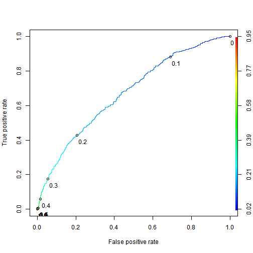
#ROCRauc = performance(ROCRpred, "auc")
ROCRauc <- as.numeric(performance(ROCRpred, "auc")@y.values)
ROCRauc
## [1] 0.6720995- ANS: 0.6720995
Explanation </br> The test set AUC can be computed with the following commands: library(ROCR) pred = prediction(test$predicted.risk, test$not.fully.paid) as.numeric(performance(pred, “auc”)@y.values)
The model has poor accuracy at the threshold 0.5. But despite the poor accuracy, we will see later how an investor can still leverage this logistic regression model to make profitable investments.
4. A “Smart Baseline”
1. In the previous problem, we built a logistic regression model that has an AUC significantly higher than the AUC of 0.5 that would be obtained by randomly ordering observations. However, LendingClub.com assigns the interest rate to a loan based on their estimate of that loan’s risk. This variable, int.rate, is an independent variable in our dataset. In this part, we will investigate using the loan’s interest rate as a “smart baseline” to order the loans according to risk. Using the training set, build a bivariate logistic regression model (aka a logistic regression model with a single independent variable) that predicts the dependent variable not.fully.paid using only the variable int.rate. The variable int.rate is highly significant in the bivariate model, but it is not significant at the 0.05 level in the model trained with all the independent variables. What is the most likely explanation for this difference?
model1 <-glm(not.fully.paid ~ int.rate, data = train, family = "binomial")
summary(model1)
##
## Call:
## glm(formula = not.fully.paid ~ int.rate, family = "binomial",
## data = train)
##
## Deviance Residuals:
## Min 1Q Median 3Q Max
## -1.0547 -0.6271 -0.5442 -0.4361 2.2914
##
## Coefficients:
## Estimate Std. Error z value Pr(>|z|)
## (Intercept) -3.6726 0.1688 -21.76 <2e-16 ***
## int.rate 15.9214 1.2702 12.54 <2e-16 ***
## ---
## Signif. codes: 0 '***' 0.001 '**' 0.01 '*' 0.05 '.' 0.1 ' ' 1
##
## (Dispersion parameter for binomial family taken to be 1)
##
## Null deviance: 5896.6 on 6704 degrees of freedom
## Residual deviance: 5734.8 on 6703 degrees of freedom
## AIC: 5738.8
##
## Number of Fisher Scoring iterations: 4- ANS: int.rate is correlated with other risk-related variables, and therefore does not incrementally improve the model when those other variables are included.
Explanation </br> To train the bivariate model, run the following command: bivariate = glm(not.fully.paid~int.rate, data=train, family=”binomial”) summary(bivariate)
Decreased significance between a bivariate and multivariate model is typically due to correlation. From cor(train$int.rate, train$fico), we can see that the interest rate is moderately well correlated with a borrower’s credit score.
Training/testing set split rarely has a large effect on the significance of variables (this can be verified in this case by trying out a few other training/testing splits), and the models were trained on the same observations.
2. Make test set predictions for the bivariate model. What is the highest predicted probability of a loan not being paid in full on the testing set?
smartPred <- predict(model1, newdata = test, type = "response")
summary(smartPred)
## Min. 1st Qu. Median Mean 3rd Qu. Max.
## 0.06196 0.11550 0.15080 0.15960 0.18930 0.42660# max(summary(smartPred))- ANS: 0.4266
- With a logistic regression cutoff of 0.5, how many loans would be predicted as not being paid in full on the testing set?
table(test$not.fully.paid, smartPred > 0.5)##
## FALSE
## 0 2413
## 1 460- ANS: 0
Explanation </br> Make and summarize the test set predictions with the following code:
pred.bivariate = predict(bivariate, newdata=test, type=”response”)
summary(pred.bivariate)
According to the summary function, the maximum predicted probability of the loan not being paid back is 0.4266, which means no loans would be flagged at a logistic regression cutoff of 0.5.
3. What is the test set AUC of the bivariate model?
ROCRsmartpred = prediction(smartPred, test$not.fully.paid)
ROCRsmartperf = performance(ROCRsmartpred, "tpr", "fpr")
plot(ROCRsmartperf, colorize=TRUE)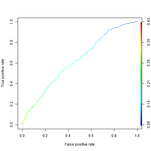
#ROCRsmartauc = performance(ROCRsmartpred, "auc")
ROCRsmartauc = performance(ROCRsmartpred, "auc")@y.values
#ROCRsmartauc- ANS: 0.6239081
Explanation </br> The AUC can be computed with: prediction.bivariate = prediction(pred.bivariate, test$not.fully.paid) as.numeric(performance(prediction.bivariate, “auc”)@y.values)
5. Computing the Profitability of an Investment
While thus far we have predicted if a loan will be paid back or not, an investor needs to identify loans that are expected to be profitable. If the loan is paid back in full, then the investor makes interest on the loan. However, if the loan is not paid back, the investor loses the money invested. Therefore, the investor should seek loans that best balance this risk and reward. To compute interest revenue, consider a $c investment in a loan that has an annual interest rate r over a period of t years. Using continuous compounding of interest, this investment pays back c * exp(rt) dollars by the end of the t years, where exp(rt) is e raised to the r*t power. </br> How much does a $10 investment with an annual interest rate of 6% pay back after 3 years, using continuous compounding of interest? Hint: remember to convert the percentage to a proportion before doing the math. Enter the number of dollars, without the $ sign. </br>
10*exp(0.06*3)## [1] 11.97217Explanation </br> In this problem, we have c=10, r=0.06, and t=3. Using the formula above, the final value is 10exp(0.063) = 11.97.
6. A Simple Investment Strategy
In the previous subproblem, we concluded that an investor who invested c dollars in a loan with interest rate r for t years makes c * (exp(rt) - 1) dollars of profit if the loan is paid back in full and -c dollars of profit if the loan is not paid back in full (pessimistically). In order to evaluate the quality of an investment strategy, we need to compute this profit for each loan in the test set. For this variable, we will assume a $1 investment (aka c=1). To create the variable, we first assign to the profit for a fully paid loan, exp(rt)-1, to every observation, and we then replace this value with -1 in the cases where the loan was not paid in full. All the loans in our dataset are 3-year loans, meaning t=3 in our calculations. Enter the following commands in your R console to create this new variable:
test$profit = exp(test$int.rate*3) - 1
test$profit[test$not.fully.paid == 1] = -1
# max(test$profit)*10
ans <- max(test$profit)*10-
What is the maximum profit of a $10 investment in any loan in the testing set (do not include the $ sign in your answer)? </br>
-
ANS 8.8947687
Explanation </br> From summary(test$profit), we see the maximum profit for a $1 investment in any loan is $0.8895. Therefore, the maximum profit of a $10 investment is 10 times as large, or $8.895. summary(test$profit)
6. An Investment Strategy Based on Risk
1. A simple investment strategy of equally investing in all the loans would yield profit $20.94 for a $100 investment. But this simple investment strategy does not leverage the prediction model we built earlier in this problem. As stated earlier, investors seek loans that balance reward with risk, in that they simultaneously have high interest rates and a low risk of not being paid back. To meet this objective, we will analyze an investment strategy in which the investor only purchases loans with a high interest rate (a rate of at least 15%), but amongst these loans selects the ones with the lowest predicted risk of not being paid back in full. We will model an investor who invests $1 in each of the most promising 100 loans. First, use the subset() function to build a data frame called highInterest consisting of the test set loans with an interest rate of at least 15%. </br> What is the average profit of a $1 investment in one of these high-interest loans (do not include the $ sign in your answer)?
highInterest  <- subset(test, test$int.rate  >= 0.15)
# mean(highInterest$profit)
# sum(highInterest$not.fully.paid == 1)/nrow(highInterest)- ANS: 0.2251015
What proportion of the high-interest loans were not paid back in full?
- ANS: 0.2517162
Explanation </br> The following two commands build the data frame highInterest and summarize the profit variable. highInterest = subset(test, int.rate >= 0.15) summary(highInterest$profit) We read that the mean profit is $0.2251. To obtain the breakdown of whether the loans were paid back in full, we can use table(highInterest$not.fully.paid) 110 of the 437 loans were not paid back in full, for a proportion of 0.2517.
2. Next, we will determine the 100th smallest predicted probability of not paying in full by sorting the predicted risks in increasing order and selecting the 100th element of this sorted list. Find the highest predicted risk that we will include by typing the following command into your R console:
cutoff = sort(highInterest$predicted.risk, decreasing=FALSE)[100]Use the subset() function to build a data frame called selectedLoans consisting of the high-interest loans with predicted risk not exceeding the cutoff we just computed. Check to make sure you have selected 100 loans for investment.
What is the profit of the investor, who invested $1 in each of these 100 loans (do not include the $ sign in your answer)?
selectedLoans = subset(highInterest, predicted.risk <= cutoff)
dim(selectedLoans)
## [1] 100 16# sum(selectedLoans$profit)- ANS: 31.2782493
How many of 100 selected loans were not paid back in full?
table(selectedLoans$not.fully.paid)##
## 0 1
## 81 19# sum(selectedLoans$not.fully.paid == 1)- ANS: 19