
Singular Value Decomposition and Image Processing
23 Jun 2015The singular value decomposition (SVD) is a factorization of a real or complex matrix. It has many useful applications in signal processing and statistics.
Singular Value Decomposition
SVD is the factorization of a \( m \times n \) matrix \( Y \) into three matrices as:
With:
- \( U \) is an \( m\times n \) orthogonal matrix
- \( V \) is an \( n\times n \) orthogonal matrix
- \( D \) is an \( n\times n \) diagonal matrix
In R The result of svd(X) is actually a list of three components named d, u and v, such that Y = U %*% D %*% t(V).
Video about SVD
</embed>
Example
# cleanup
rm(list=ls())

dat <- seq(1,36,2)

Y <- matrix(dat,ncol=6)
Y
## [,1] [,2] [,3] [,4] [,5] [,6]
## [1,] 1 7 13 19 25 31
## [2,] 3 9 15 21 27 33
## [3,] 5 11 17 23 29 35# Apply SVD to get U, V, and D
s <- svd(Y)
U <- s$u
V <- s$v
D <- diag(s$d) ##turn it into a matrix- we can reconstruct Y
Yhat <- U %*% D %*% t(V)
Yhat
## [,1] [,2] [,3] [,4] [,5] [,6]
## [1,] 1 7 13 19 25 31
## [2,] 3 9 15 21 27 33
## [3,] 5 11 17 23 29 35resid <- Y - Yhat
max(abs(resid))## [1] 2.309264e-14Image processing
- Load the image and convert it to a greyscale:
# source("http://bioconductor.org/biocLite.R")
# biocLite("ripa", dependencies=TRUE)
# biocLite("rARPACK", dependencies=TRUE)
# install.packages('devtools')
# library(devtools)
# install_github('ririzarr/rafalib')

# Load libraries
library(rARPACK)
library(ripa)    #  function "imagematrix"
library(EBImage)
library(jpeg)
library(png)
#
library(rafalib)
mypar2()
#
# Read the image
img <- readImage("images/pansy.jpg")
dim(img)
## [1] 465 600 3display(img, method = "raster")
# Convert image to greyscale
r <- imagematrix(img, type = "grey")

# display(r, method = "raster", all=TRUE)
display(r, method = "raster")
dim(r)## [1] 465 600str(r)## imagematrix [1:465, 1:600] 0.345 0.282 0.29 0.306 0.29 ...
## - attr(*, "type")= chr "grey"
## - attr(*, "class")= chr [1:2] "imagematrix" "matrix"- Apply SVD to get U, V, and D
# Apply SVD to get u, v, and d
r.svd <- svd(r)

u <- r.svd$u
v <- r.svd$v
d <- diag(r.svd$d)
dim(d)
## [1] 465 465## [1] 465 465- Plot the magnitude of the singular values
# check svd$d values
# Plot the magnitude of the singular values
sigmas = r.svd$d # diagonal matrix (the entries of which are known as singular values)
plot(1:length(r.svd$d), r.svd$d, xlab="i-th r.svd$d", ylab="r.svd$d",  main="Singular Values");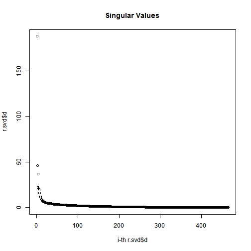
plot(1:length(r.svd$d), cumsum(r.svd$d) / sum(r.svd$d), main="Cumulative Percent of Total Sigmas");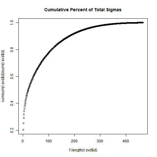 Not that, the total of the first n singular values divided by the sum of all the singular values is the percentage of “information” that those singular values contain. If we want to keep 90% of the information, we just need to compute sums of singular values until we reach 90% of the sum, and discard the rest of the singular values.
# first approximation
u1 <- as.matrix(u[-1, 1])
v1 <- as.matrix(v[-1, 1])
d1 <- as.matrix(d[1, 1])
l1 <- u1 %*% d1 %*% t(v1)
l1g <- imagematrix(l1, type = "grey")
#plot(l1g, useRaster = TRUE)
display(l1g, method = "raster", all=TRUE)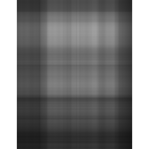
# more approximation
depth <- 5
us <- as.matrix(u[, 1:depth])
vs <- as.matrix(v[, 1:depth])
ds <- as.matrix(d[1:depth, 1:depth])
ls <- us %*% ds %*% t(vs)
lsg <- imagematrix(ls, type = "grey")

## Warning: Pixel values were automatically clipped because of range over.

#plot(lsg, useRaster = TRUE)
display(lsg, method = "raster")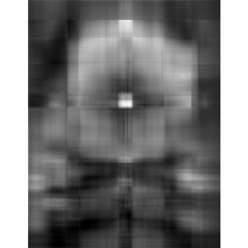
# more approximation
depth <- 20
us <- as.matrix(u[, 1:depth])
vs <- as.matrix(v[, 1:depth])
ds <- as.matrix(d[1:depth, 1:depth])
ls <- us %*% ds %*% t(vs)
lsg <- imagematrix(ls, type = "grey")

## Warning: Pixel values were automatically clipped because of range over.

#plot(lsg, useRaster = TRUE)
display(lsg, method = "raster")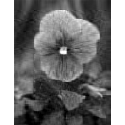
Image Compression with the SVD
Here we continue to show how the SVD can be used for image compression (as we have seen above).
factorize = function(m, k){
  r = svds(m[, , 1], k);
  g = svds(m[, , 2], k);
  b = svds(m[, , 3], k);
  return(list(r = r, g = g, b = b));
}

recoverimg = function(lst, k){
  recover0 = function(fac, k){
    dmat = diag(k);
    diag(dmat) = fac$d[1:k];
    m = fac$u[, 1:k] %*% dmat %*% t(fac$v[, 1:k]);
    m[m < 0] = 0;
    m[m > 1] = 1;
    return(m);
  }

  r = recover0(lst$r, k);
  g = recover0(lst$g, k);
  b = recover0(lst$b, k);
  m = array(0, c(nrow(r), ncol(r), 3));
  m[, , 1] = r;
  m[, , 2] = g;
  m[, , 3] = b;
  return(m);
}

rawimg <- readJPEG("images/pansy.jpg");

lst = factorize(rawimg, 100);

neig = c(1, 5, 20, 50, 100);
for(i in neig){
  m = recoverimg(lst, i);
  writeJPEG(m, sprintf("images/svd_%d.jpg", i), 0.95);
  #display(m, method = "raster")
  fname <- sprintf("images/svd_%d.jpg", i)
  display(readImage(fname), title="svd_%d", method = "raster")
}- Original image
- Singluar Value k = 1
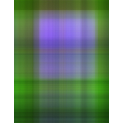
- Singluar Value k = 5
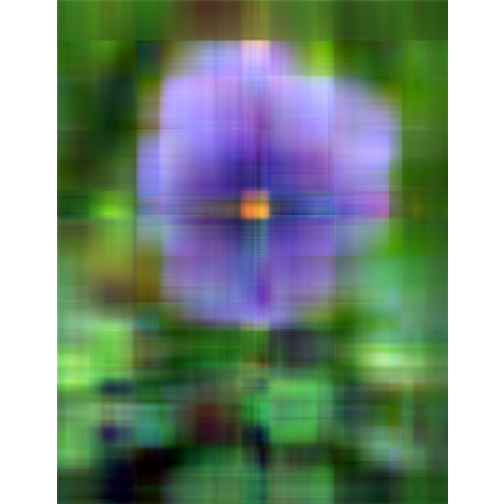
- Singluar Value k = 20
- Singluar Value k = 50

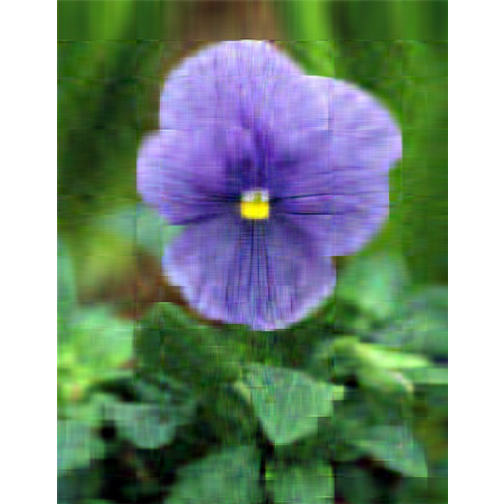
-
Singluar Value k = 100

- Analysis
With only 10% of the real data we are able to create a very good approximation of the real data.
References
- http://www.omgwiki.org/hpec/files/hpec-challenge/svd.html
- http://andrew.gibiansky.com/blog/mathematics/cool-linear-algebra-singular-value-decomposition
- https://en.wikipedia.org/wiki/Singular_value_decomposition
- http://genomicsclass.github.io/book/pages/svd.html
- https://en.wikibooks.org/wiki/Data_Mining_Algorithms_In_R/Dimensionality_Reduction/Singular_Value_Decomposition
- http://emma.memect.com/t/1acca3994986f1f736c81a0daf5fa3c3949ea2a8d8962453ed5ba826bb461ac5/Data%20Mining%20Algorithms%20In%20R.pdf
- https://github.com/ralphbrooks/datascience
- https://gist.github.com/casunlight/9628504
- http://blog.translucentcomputing.com/2014/03/principal-component-analysis-for.html
- http://www.ats.ucla.edu/stat/r/pages/svd_demos.htm
- http://www.r-bloggers.com/image-compression-with-the-svd-in-r/