
Map Visualization in R
10 Jun 2015Here I tried to produce some map visualization in R.
- First using data from GADM database of Global Administrative Areas.
- Second using the package RWorldMap,
- Third using the package ggmap that allows visualizations of spatial data on maps retrieved from Google Maps, OpenStreetMap, etc., and
- Fourth using the package RgoogleMaps allows you to plot data points on any kind of map you can imagine (terrain, satellite, hybrid).
1. Data from GADM database
Getting the spatial country data
library(geosphere) # use: gcIntermediate
library(RgoogleMaps); library(ggmap); library(rworldmap)
library(sp); library(maptools); require(RColorBrewer)

# PRT_adm2.RData download from http://www.gadm.org/
# load("data/PRT_adm2.RData") # Creates and stores in memory an object called ´gadm´
# or:
# con <- url("http://biogeo.ucdavis.edu/data/gadm2/R/PRT_adm1.RData")
# print(load(con))
# close(con)
# or:
# library(raster)
# port1 <- getData('GADM', country='PRT', level=1)

load("data/PRT_adm1.RData")
port1 <- get("gadm")
Plot the map
We can use the variable NAME_1 to plot the map:
# Convert the encoding to UTF-8 in order to avoid the problems with 'accents'.
# port1$NAME_1 <- as.factor(iconv(as.character(port1$NAME_1), , "UTF-8"))
port1$NAME_1 <- as.factor(as.character(port1$NAME_1))

spplot(port1, "NAME_1",
       col.regions = colorRampPalette(brewer.pal(12, "Set3"))(18),
       col = "white",
       #cex=0.4,
       xlim = range(-10,-6), ylim = range(36.9,42.2), asp = 1.0
       #scales=list(draw=TRUE)
       )  # Plot the 'NAME_1' form the 'port1' object.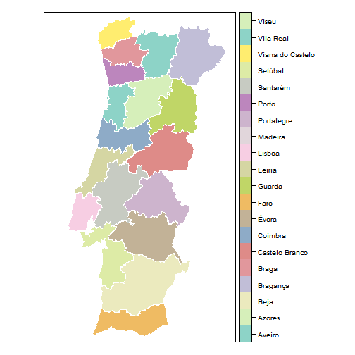
And next we created another variable called rainfall in the data.frame, we store random values in that variable:
set.seed(333)
port1$rainfall<-rnorm(length(port1$NAME_1),mean=50,sd=15) #random rainfall value allocation

spplot(port1,"rainfall",col.regions = rev(terrain.colors(port1$rainfall)),
       scales=list(draw=TRUE),
       main="Rainfall (simulated) in Portugal")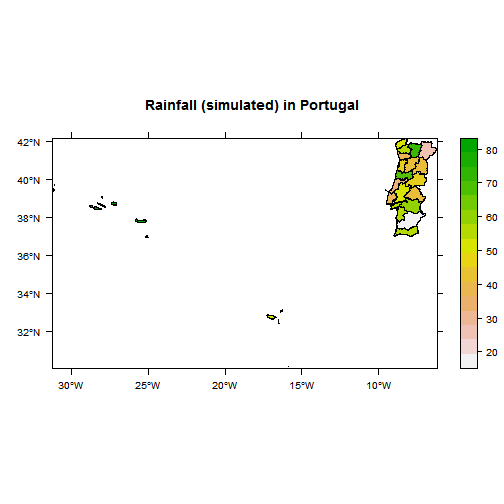
2. RWorldMap
Rworldmap is a package for visualising global data, referenced by country. It provides maps as spatial polygons.
newmap <- getMap(resolution = "low")
plot(newmap)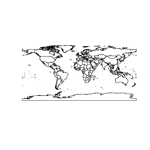
By Changing the xlim and ylim arguments of the plot function we can limit the display to just Europe.
plot(newmap, xlim = c(-20, 59), ylim = c(35, 71), asp = 1 )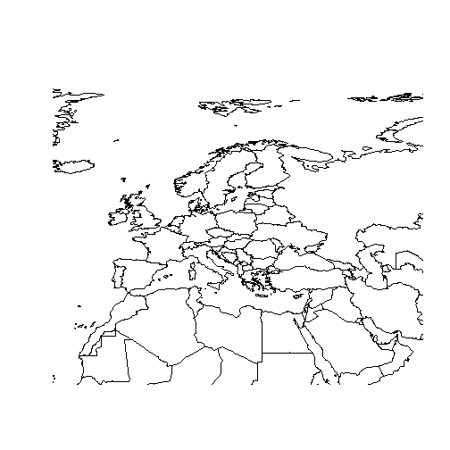
Geocoding
The geocode function from the ggmap package finds the coordinates of a location using Google Maps. Thus, finding the coordinates of the Extreme points of Europe can be done by:
europe.limits <- geocode(c("CapeFligely,RudolfIsland,Franz Josef Land,Russia",
                           "Gavdos,Greece", "Faja Grande,Azores",
                           "SevernyIsland,Novaya Zemlya,Russia"))
europe.limits
## lon lat
## 1 60.64878 80.58823
## 2 24.08464 34.83469
## 3 -31.26192 39.45479
## 4 56.00000 74.00000So we can display only the europe as follow, by modifying the xlim and ylim arguments:
plot(newmap, xlim = range(europe.limits$lon), ylim = range(europe.limits$lat), asp = 1)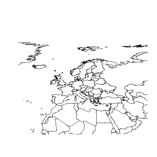
3. ggmap
- Fetching a Map
# geocodes
geoCodes <- geocode("Portela,2230")
geoCodes
## lon lat
## 1 -8.250595 39.61002# lon lat
# 1 -8.250595 39.61002ggmap(
get_googlemap(
center=c(geoCodes$lon,geoCodes$lat), #Long/lat of centre
zoom=14,
maptype='satellite', #also hybrid/terrain/roadmap
scale = 2), #resolution scaling, 1 (low) or 2 (high)
size = c(600, 600), #size of the image to grab
extent='device', #can also be "normal" etc
darken = 0) #you can dim the map when plotting on top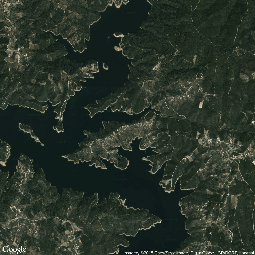
#ggsave ("images/map1.png", dpi = 200) #this saves the output to a file- Plotting on a Map
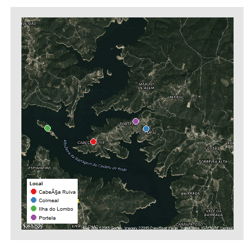
You can plot any [x,y, +/- z] information you’d like on top of a ggmap, so long as x and y correspond to longitudes and latitudes within the bounds of the map you have fetched. To plot on top of the map you must first make your map a variable and add a geom layer to it.
#Generate some data
#         lat        lon
# Colmeal 39.609025, -8.245660
# Portela 39.610447, -8.248321
# Cabeça_Ruiva 39.606380, -8.259393
# Ilha_do_Lombo 39.609124, -8.271237
long = c(-8.245660, -8.248321, -8.259393, -8.271237)
lat = c(39.609025, 39.610447, 39.606380, 39.609124)
who = c("Colmeal", "Portela", "Cabeça Ruiva", "Ilha do Lombo")
data = data.frame (long, lat, who)

map = ggmap(
    get_googlemap(
		center=c(geoCodes$lon,geoCodes$lat),
		zoom=14,
		maptype='hybrid',
		scale = 2),
		size = c(600, 600),
		extent='normal',
		darken = 0)

map + geom_point (
		data = data,
		aes (
			x = long,
			y = lat,
			fill = factor (who)
			),
		pch = 21,
		colour = "white",
		size = 6
		) +

	scale_fill_brewer (palette = "Set1", name = "Local") +

	#for more info on these type ?theme()
	theme (
		legend.position = c(0.05, 0.05), # put the legend INSIDE the plot area
		legend.justification = c(0, 0),
		legend.background = element_rect(colour = F, fill = "white"),
		legend.key = element_rect (fill = F, colour = F),
		panel.grid.major = element_blank (), # remove major grid
		panel.grid.minor = element_blank (),  # remove minor grid
		axis.text = element_blank (),
		axis.title = element_blank (),
		axis.ticks = element_blank ()
) 
#ggsave (""images/map2.png"", dpi = 200)4. RgoogleMaps
‘RgoogleMaps’ allows you to plot data points on any kind of map you can imagine (terrain, satellite, hybrid).
lat <- c(37,42) #define our map's ylim
lon <- c(-9,-6) #define our map's xlim
lat <- c(37,42) #define our map's ylim
lon <- c(-12,-6) #define our map's xlim
center = c(mean(lat), mean(lon))  #tell what point to center on
zoom <- 7  #zoom: 1 = furthest out (entire globe), larger numbers = closer in

# get maps from Google
terrmap <- GetMap(center=center, zoom=zoom, maptype= "terrain", destfile = "terrain.png")
# visual options:
#   maptype = c("roadmap", "mobile", "satellite", "terrain", "hybrid", "mapmaker-roadmap", "mapmaker-hybrid")
PlotOnStaticMap(terrmap)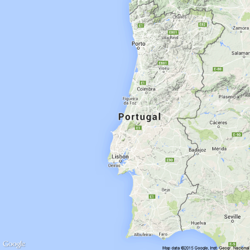
# Sard <- geocode("Sardoal, PT") # find coordinates
# Sard
#         lon      lat
# 1 -8.161277 39.53752

# using maps to plot routes
rt1 = route(from = "Lisbon", to = "Castelo Branco", mode = "driving")
rt2 = route(from = "Lisbon", to = "Sardoal", mode = "driving")
rt3 = route(from = "Abrantes", to = "Castelo Branco", mode = "driving")

PortugalMap <- qmap("Portugal", zoom = 8, color = "bw")

PortugalMap + geom_leg(aes(x = startLon, y = startLat, xend = endLon, yend = endLat),
                       color = "blue", data = rt1) +
    geom_leg(aes(x = startLon, y = startLat, xend = endLon, yend = endLat),
                       color = "black", data = rt2) +
    geom_leg(aes(x = startLon, y = startLat, xend = endLon, yend = endLat),
                       color = "red", data = rt3)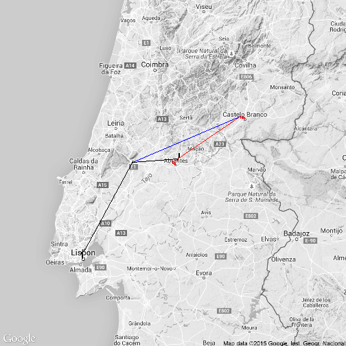
References
- OpenStreeMap
- http://www.molecularecologist.com/2012/09/making-maps-with-r/
- http://allthingsr.blogspot.pt/2012/03/geocode-and-reverse-geocode-your-data.html
- http://www.r-bloggers.com/13-mapping-in-r-representing-geospatial-data-together-with-ggplot/
- https://dl.dropboxusercontent.com/u/24648660/ggmap%20useR%202012.pdf
- https://wilkinsondarren.wordpress.com/2013/02/01/mapping-in-r-representing-geospatial-data-together-with-ggplot/
- https://www.google.pt/maps/@39.6100171,-8.2505952,15z?hl=pt-PT
- http://www.di.fc.ul.pt/~jpn/r/maps/index.html
- http://www.milanor.net/blog/?p=594
- http://pakillo.github.io/R-GIS-tutorial/