Reproducible Research - PA2
23 Apr 2015Analysis on U.S. NOAA storm database
Synopsis
Storms and other severe weather events can cause both public health and economic problems for communities and municipalities. Many severe events can result in fatalities, injuries, and property damage, and preventing such outcomes to the extent possible is a key concern.
The basic goal of this assignment is to explore the NOAA Storm Database and answer some basic questions about severe weather events. The events in the database start in the year 1950 and end in November 2011.
-
Across the United States, which types of events (as indicated in the EVTYPE variable) are most harmful with respect to population health?
-
Across the United States, which types of events have the greatest economic consequences?
Data Processing
# cleanup
rm(list=ls())
echo = TRUE # Make code visible
source("multiplot.R") # multiplot
suppressWarnings(library(plyr))
library(knitr)
suppressWarnings(library(ggplot2))
system.time(df <- read.csv(bzfile("repdata_data_StormData.csv.bz2"),
header = TRUE,
#quote = "",
strip.white=TRUE,
stringsAsFactors = FALSE))## user system elapsed
## 94.81 0.59 95.44# user system elapsed
# 469.36 3.18 656.79 << pc1
#str(df)
dim(df) # 902297 37## [1] 902297 37#colnames(df)Results
-
In this study, it’s assumed that harmful events with respect to population health comes from variables FATALITIES and INJURIES.
-
Select useful data
#
df <- df[ , c("EVTYPE", "BGN_DATE", "FATALITIES", "INJURIES", "PROPDMG", "PROPDMGEXP", "CROPDMG", "CROPDMGEXP")]
#str(df)
#dim(df) # 902297      8
#length(unique(df$EVTYPE)) # 985

#head(df$BGN_DATE)
df$BGN_DATE <- as.POSIXct(df$BGN_DATE,format="%m/%d/%Y %H:%M:%S")
#head(df$BGN_DATE)
#unique(df$PROPDMGEXP)
#unique(df$CROPDMGEXP)
#- Create new variables: TOTAL_PROPDMG, TOTAL_CROPDMG and TOTALDMG with: TOTALDMG = (TOTAL_PROPDMG + TOTAL_CROPDMG)
tmpPROPDMG <- mapvalues(df$PROPDMGEXP,
                         c("K","M","", "B","m","+","0","5","6","?","4","2","3","h","7","H","-","1","8"),
                         c(1e3,1e6, 1, 1e9,1e6,  1,  1,1e5,1e6,  1,1e4,1e2,1e3,  1,1e7,1e2,  1, 10,1e8))

tmpCROPDMG <- mapvalues(df$CROPDMGEXP,
                         c("","M","K","m","B","?","0","k","2"),
                         c( 1,1e6,1e3,1e6,1e9,1,1,1e3,1e2))
#colnames(df)
df$TOTAL_PROPDMG <- as.numeric(tmpPROPDMG) * df$PROPDMG
df$TOTAL_CROPDMG <- as.numeric(tmpCROPDMG) * df$CROPDMG
colnames(df)
## [1] "EVTYPE" "BGN_DATE" "FATALITIES" "INJURIES"
## [5] "PROPDMG" "PROPDMGEXP" "CROPDMG" "CROPDMGEXP"
## [9] "TOTAL_PROPDMG" "TOTAL_CROPDMG"remove(tmpPROPDMG)
remove(tmpCROPDMG)
df$TOTALDMG <- df$TOTAL_PROPDMG + df$TOTAL_CROPDMG
##
head(unique(df$EVTYPE))## [1] "TORNADO" "TSTM WIND" "HAIL"
## [4] "FREEZING RAIN" "SNOW" "ICE STORM/FLASH FLOOD"Population health impact
- Across the United States, which types of events (as indicated in the EVTYPE variable) are most harmful with respect to population health?
summary1 <- ddply(df,"EVTYPE", summarize, propdamage = sum(TOTALDMG), injuries= sum(INJURIES), fatalities = sum(FATALITIES), persdamage = sum(INJURIES)+sum(FATALITIES))
summary1 <- summary1[order(summary1$propdamage, decreasing = TRUE),]
#head(summary1,10)
#tmp = head(summary1,10)
summary2 <- summary1[order(summary1$persdamage, decreasing = TRUE),]
#head(summary2,10)
plot2 <- ggplot(data=head(summary2,10), aes(x=EVTYPE, y=persdamage, fill=persdamage)) +
geom_bar(stat="identity",position=position_dodge()) +
labs(x = "event type", y = "personal damage (injuries and fatalities)") +
scale_fill_gradient("personal damage", low = "lightblue", high = "darkblue") +
ggtitle("Effect of Severe Weather on Public Health") +
theme(axis.text.x = element_text(angle=90, hjust=1))
print(plot2)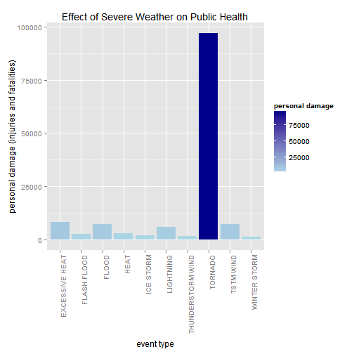 </br>
</br>
- From the above figure we can see that TORNADOES have the most significant impact on public health.
</br>
- Across the United States, which types of events have the greatest economic consequences?
##
plot1 <- ggplot(data=head(summary1,10), aes(x=EVTYPE, y=propdamage, fill=propdamage)) +
geom_bar(stat="identity",position=position_dodge()) +
labs(x = "event type", y = "property damage (in $USD)") +
scale_fill_gradient("$USD", low = "lightblue", high = "darkblue") +
ggtitle("Effect of Severe Weather on the U.S. Economy") +
theme(axis.text.x = element_text(angle=90, hjust=1))
print(plot1)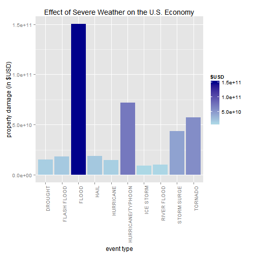 </br>
</br>
- The FLOODS, HURRICANES/TYPHOONES and TORNADOES are the events with the greatest economic consequences.
summary3 <- summary1[order(summary1$"injuries", decreasing = TRUE),]
#head(summary3,10)

plot3 <- ggplot(data=head(summary3,10), aes(x=EVTYPE, y=injuries, fill=injuries)) +
  geom_bar(stat="identity",position=position_dodge()) +
  #labs(x = "event type", y = "personal damage (injuries and fatalities)") +
  labs(x = "event type", y = "personal damage (injuries)") +
  scale_fill_gradient("injuries", low = "yellow", high = "red") +
  theme(axis.text.x = element_text(angle=90, hjust=0.8))
  #scale_fill_gradient("personal damage", low = "yellow", high = "red") +
  #theme(axis.text.x = element_text(angle=60, hjust=1))

summary4 <- summary1[order(summary1$"fatalities", decreasing = TRUE),]
#head(summary4,10)

plot4 <- ggplot(data=head(summary4,10), aes(x=EVTYPE, y=fatalities, fill=fatalities)) +
  geom_bar(stat="identity",position=position_dodge()) +
  labs(x = "event type", y = "personal damage (fatalities)") +
  scale_fill_gradient("fatalities", low = "yellow", high = "red") +
  theme(axis.text.x = element_text(angle=90, hjust=0.8))
#print(plot3)
#print(plot4)
multiplot(plot3, plot4, cols=2)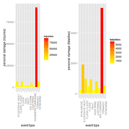
#</br>
- TORNADO is the harmful event with respect to population health, and
- FLOOD is the event which have the greatest economic consequences.